Material on this page is copyright © 2020 John W.F. Waldron
Dynamic analysis is concerned with force and stress (force per unit area).
The first word in dealing with stress is caution! Beginners in geology, encouraged in some cases by poorly worded textbooks, are apt to jump to dynamic conclusions based on observations of geometry. Despite many decades of research in structural geology, it is unusual to be able to make any quantitative deductions about stress from outcrop observations!
Part of the problem is that geological strain rates for ductile deformation are very slooooooooow, so we cannot directly determine what kind of stress makes what kind of structure, unless we are prepared to run our experiments for 10,000 years or more! For brittle deformation, experimental simulation of structures is easier, but experimental structural geology is still a challenging field.
That said, understanding of stress is critically important in areas of structural geology and engineering that deal with stress at the present day, such as earthquake studies, and the behaviour of fluids (water, oil, gas) in the subsurface, so we do need to know how stress is measured, and the potential ways that structures are related to stress.
The concentration force on any plane can be expressed in Nm-2 or Pa. This quantity is a vector with three components, commonly known as stress.
Note: the word stress used in two ways. It can describe the force concentration on a plane, also known as traction, (or, in the special case where the force is perpendicular to the plane, as pressure). However, it can also be used to describe the array of forces that act on all possible planes that pass through a point. This 3D state of stress cannot be described by a single vector - it is a tensor quantity. Some textbooks restrict the word stress to this tensor quantity, and use the word traction to for the vector that describes force concentration on a single plane. In these notes, the term 'stress' is used informally for both the tensor quantity and its vector manifestation. If there is any possibility of confusion, we will write 'stress on a plane' or 'stress tensor' to distinguish the two concepts.
In formulas, the common convention is to use the greek letter sigma σ for the stress vector. Tensors are usually represented by uppercase bold letters, but uppercase sigma (Σ) is used for too many other things! We will use an uppercase T if we need to represent the stress tensor algebraically.
The component of stress σn perpendicular to a surface is the normal stress (or traction).
The part of the stress σs or τ parallel to a surface is called the shear stress (or traction). The overall stress on the surface is equal to the vector sum of the normal and shear stress.
Shear stress can itself be resolved into components parallel (for example) to the strike and the dip of the surface.
Note that in geology we normally regard compressive normal stresses as positive, because compressive stresses are much more common in the Earth. (This leads to some difficulties when we relate stress and strain, because we treat extensional strains as positive, and shortening as negative.)
The SI unit of stress is the pascal, equal to one Newton per square metre. However, even a gentle breeze exerts several pascals of stress on the Earth's surface, so 1 pascal doesn't do much to the average rock. Geologists have used a confusing variety of alternative stress measures:
To give a general idea of the range of crustal stresses, the mean stress (roughly equivalent to pressure) at the base of the continental crust is around 1 GPa, 10 kb, 10000 atm, or 14500 psi.
As we move into 3-D things get complicated. At any point inside the Earth there is an infinite number of differently oriented surfaces. In a liquid, these surfaces all experience the same stress and we describe the state of stress with a single number, the pressure.
In a solid, each plane will experience a different stress vector
If we draw all the vectors describing the stress at a point, they will define a stress ellipsoid. It's a graphic representation but not a very convenient tool for doing stress calculations.
It turns out that we can completely specify the state of stress at a point within the earth can be thought of as acting on the surfaces of a tiny cube.
While the cube is stationary, forces on opposite faces must be equal and opposite, so there are three surfaces, with nine stress components, to consider. The nine components can be represented by a matrix, the stress tensor
Arguments involving moments can be used to show that σ12 = σ21 etc, so the matrix is symmetric and there are only six independent components.
The stress tensor is a much more practical means of representing the stress because it can be used to calculate the traction on any arbitrarily oriented plane, if that plane can be represented by a unit vector â. The calculation is a matrix multiplication.
σ = Tâ
In general there will be three special mutually perpendicular planes, that suffer no shear stress, only normal stress.
The poles to these planes are the stress axes, and the stresses that act along them are called principal stresses. σ1 >σ2 >σ3.
This means that the stress on the plane acts in the same direction as the pole to the plane. Hence, mathematically, the stress vector is a simple multiple of the vector that represents the plane:
σ = kâ = Tâ
Where k is a scalar constant. This equation is actually the definition of an eigenvector - a concept we met in the section on statistics.
So, the stress axes correspond to the eigenvectors of the stress tensor.
If the stress axes 1, 2, and 3 happen to coincide with the coordinate axes 1, 2, and 3 then the stress tensor becomes very simple..
If two of the principal stresses are zero, then the state of stress is described as uniaxial.
If one of the principal stresses is zero, and two are non-zero, then the stress is biaxial.
If all three principal stresses are non-zero (even if two or three are the same) then the stress state is triaxial.
If we take the average of the magnitudes of the three principle stresses, we are finding the mean stress which is equivalent to the normal concept of pressure (e.g. in metamorphic petrology).
Mean stress σm = (σ1 + σ2 + σ3)/3
The rest of the stress, which we get by subtracting the mean stress from the three diagonal components of the stress tensor, is called the deviatoric or differential stress.
Deviatoric stress =
An easy way to think about the mean and deviatoric stress components is to consider that
Another useful measure of the part of the stress that acts to change shape is just the difference between the maximum and minimum principal stresses.
Differential stress σd = (σ1 - σ3)
This measure is very useful in studies of fracture formation, and any situation where the value of the intermediate principal stress is less important than the two extremes
Sometimes part of the mean stress in a rock is supported by pore fluid pressure. This reduces the effect of normal stresses on the mineral grains, effectively reducing the mean stress, but leaves the shear stresses unaffected.
The effective stress (or effective pressure) is defined as the stress minus the pore fluid pressure.
Standared states of stress are those where stress is due entirely to gravity acting on the rocks of the lithosphere.
The hydrostatic and lithostatic states of stress are the most simple, in which all three principal stresses are equal σ1 = σ2 = σ3. Under these circumstances the stress ellipsoid is a sphere and the directions of the stress axes are undefined.
Hydrostatic stress describes the situation in a water body at rest. Because water is virtually incompressible all surfaces 'feel' the same stress σ1 = σ2 = σ3 = ρgz where ρ is the density of water, g is the acceleration due to gravity, and z is the depth. If the water in a porous rock unit is in continuous connection with the surface, the pressure in that fluid is likely to be approximately hydrostatic.
Lithostatic stress is similar, but due to the density of overlying rock, not water. It's an appropriate description for parts of the crust that have remained stable under their own weight for long periods of geologic time; slow ductile deformation has allowed them to behave like a heavy fluid.
The Uniaxial-strain state of stress is an adjusted state of stress that resembles the lithostatic state but takes into account the fact that rocks are compressible. Therefore, the effect of the weight of overlying rock is to cause compaction. Because of compaction vertical surfaces do not 'feel' as much stress as horizontal surfaces.
In theory, the reduction in the horizontal stress is a function of Poisson's ratio ν, a measure of compressibility that we will meet shortly.
In practice, the state of stress in most sedimentary basins undergoing compaction is somewhere between the uniaxial strain state and the lithostatic state.
(Note: the word "uniaxial" is used differently in stress and strain studies. Uniaxial strain describes a situation where two of the principal strains are equal; in uniaxial stress two of the principal stresses are zero.)
In general, within the Earth, the stress axes σ1σ2 σ3 do not coincide with the spatial axes, though at the Earth's surface, one of the stress axes always roughly coincides with the vertical axis "z". This is because the Earth's surface is approximately horizontal and is a surface of zero shear stress (neglecting the rather small shear stresses imposed by flowing water and air.)
This principle was first put forward by Anderson, and a state of stress in which one principal stress is vertical is often described as Andersonian. There are three Andersonian regimes of stress, each characterized by a particular distribution of faults.
It's possible to calculate the stress on any surface (known as the resolved stress or traction) by geometrical constructions, but if the stress tensor is known, it is easier by matrix multiplication.
For linear algebraists, if the state of stress is represented by the stress tensor Τ, and â is a vector representing the pole to a plane, then the stress vector σ on that plane is calculated by matrix multiplication
σ = Τâ
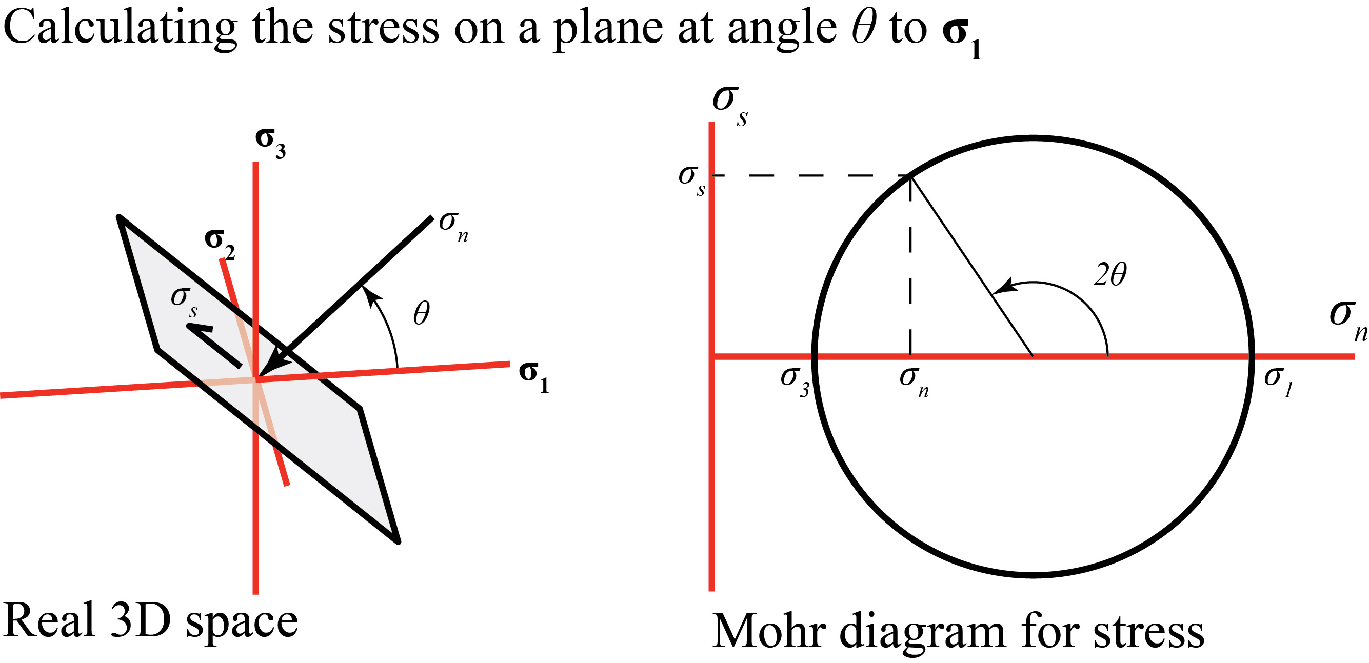
There is a Mohr circle construction for stress, which effectively carries out the tensor calculation graphically.
If normal stress is plotted on the x-axis of a graph, and shear stress is plotted on the y-axis, then all possible combinations of normal and shear stress fall inside a circle, that crosses the x axis at σ1 and σ3
If we restrict attention to planes parallel to σ2 then the combinations of normal and shear stress lie on the circle itself. The highest stresses always fall on these planes, so this is a useful diagram for predicting fractures.
It's possible to use it to predict the orientation of the plane that first exceeds the failure strength of the rock.
The conditions for brittle failure are represented by a failure envelope. When the differential stress becomes large enough, the Mohr circle intersects the failure envelope and fracture occurs.
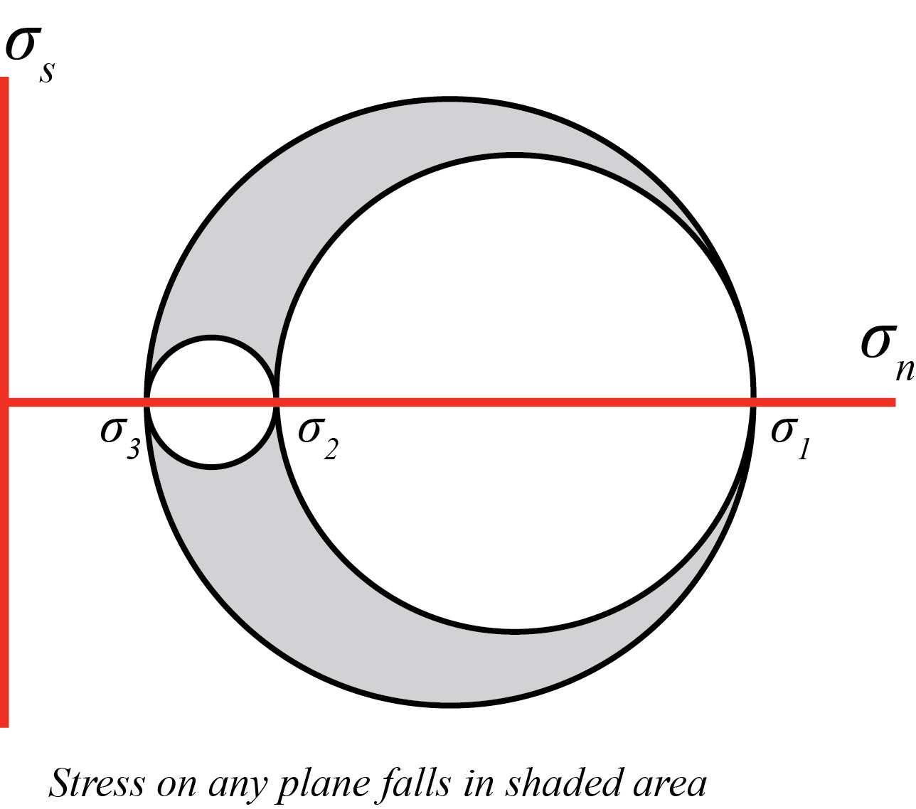
For other orientations of planes a 3D Mohr diagram is needed; it consists of 3 Mohr circles, one each for planes parallel to σ1, σ2, σ3.
The next sections are about the different ways in which rock materials respond to stress. A variety of laboratory rigs exist for stress testing materials.
Laboratory stress-testing apparatus is usually set up so that:
Elastic behaviour is the simplest response, in which strain is proportional to applied stress.
In this case, if the stress decreases, the strain decreases too, so we say elastic strain is recoverable. This type of strain is very important for understanding seismic waves and for geological engineering applications. Natural elastic strains in rocks are small and are not preserved in ancient rocks. Nonetheless it's important to understand elastic strain as it helps to determine the state of stress in the lithosphere.
Hooke's Law: In elastic deformation, the finite strain is related to stress in a proportional way.
The stress-strain relationship in one dimension for an elastic material is
normal stress σn = E.e
where E is Young's modulus of elasticity and e is the extension or fractional change in length.
Most rocks when subjected to a compressive stress in one direction will tend to expand at right angles to this direction. This tendency is expressed by Poisson's ratio ν, the ratio of thickening to shortening when stressed in this way.
Poisson's ratio ν= - ex / ez
Where ez is the extension parallel to σ1 and ex is the extension perpendicular to σ1.
For a sample that retains constant volume, the Poisson's ratio will be 0.5. Most rocks show a negative change in volume when uniaxially stressed, and therefore show Poisson's ratio between 0.5 and 0.
For an isotropic elastic material, it turns out that Young's modulus and Poisson's ratio are all that's necessary to describe the elastic properties. Though other moduli are sometimes used, they can be derived from these two quantities.
Most rocks near the Earth's surface, subjected to increasing differential stress, will eventually fail by brittle fracture. When failure occurs, the strength of the rock falls to zero across the plane of fracture. This is called loss of cohesion.
Fractures may form in several ways. In some cases, the two sides of the fracture move apart. Such fractures are known as extensional or tensile fractures; in rock outcrops the corresponding features are joints. They typically form perpendicular to the minimum principal stress σ3.
Alternatively, we may see fractures in which the two sides have moved past each other: i.e. movement is parallel to the fracture plane. These are known as shear fractures; the corresponding features in outcrops are faults. They typically form in mirror-image sets that intersect along σ2 and make some angle θ on either side of σ3. The sense of shear is such that wedge shaped blocks of rock, with their acute angle bisected by σ2, are pushed inward towards the centre of the sample. Such fractures are known as conjugate fractures.
Griffith cracks - microscopic cracks, mostly along grain boundaries - are present in all geological materials. Experimental work shows that these are important in the development of faults, because high stress concentrations occur at crack ends.
Griffith cracks oriented at high angles to σ3 tend to open as differential stress increases. In non-porous rocks, the first sign of imminent faulting may be a small volume increase called dilatancy. At depth, this volume increase is opposed by the confining pressure, and fault development is more difficult.
Stress is concentrated at the tips of the Griffith cracks, which causes them to grow. A zone of crack opening is known as a process zone or frictional breakdown zone.
Eventually, Griffith cracks join up to form a through-going fracture, along which slip can begin.
Once slip has begun, the fracture propagates extremely fast: velocities are comparable to those of seismic waves, measured in kilometres per second. It may take only milliseconds for a crack to propagate through a test sample. Naturally occurring faults in the Earth propagate over much larger distances. Natural earthquakes may last for minutes as a fracture propagates along a fault plane.
At any instant during propagation a fracture is bounded by a tip line.
Fractures may propagate as
The condition for failure can be represented on the Mohr diagram for stress by a failure envelope. Several different formulas for the failure envelope have been proposed.
The simplest was suggested by Coulomb and is a straight-line relationship between shear-stress and normal stress acting on the plane that fractures.
σs = C + σn tan φ
where φ is known as the angle of internal friction, and the constant C is the cohesion.
The Mohr construction can be used to show that this predicts that shear fractures will form such that the fracture pole makes an angle with σ1 given by:
θ = 45° + φ/2
High pore fluid pressures have the effect of reducing all the normal stresses; the shear stresses are not affected. The remaining stress, is known as the effective stress.
In the Mohr diagram, this can be shown by sliding the Mohr circle to the left, by an amount equal to the fluid pressure.
As a result of increasing the fluid pressure, the Mohr circle may intersect the failure envelope, leading to hydraulic fractures.
If the Mohr circle intersects the sloping part of the failure envelope, conjugate shear fractures are produced (Mode 2 or 3)
If the Mohr circle first intersects the part of the failure envelope in the tensile part of the diagram (σn negative), then the hydraulic fractures are Mode 1, extensional fractures
Byerlee derived an empirical relationship for movement on pre-existing fractures
Notice how under "Byerlee's law" the failure envelope does not extend into the tensile field on the left of the diagram. This means that the rock cannot sustain any tensile stress - it has no cohesion.
σs = 0.85σn ( for σn < 200 MPa)
σs = 50 MPa + 0.60σn ( for σn > 200 MPa)
Many brittle fractures occur as discrete planes, but in some rock units the grains move independently or there are multiple anastomosing fractures, that create the appearance of continuous deformation.
These types of flow may have a significant effect on porosity.
It is difficult to impossible to measure stress directly. Most methods of measuring stress actually measure the effect of stress on some material - the strain. Typically we try to choose a material for which the relationship between stress and strain (the constitutive equation) is very well known.
There are only a few methods for the direct measurement of stress in the Earth at present day. However, the present state of stress is important in petroleum production because it partially determines whether fractures are held open.
In all these methods, we actually measure an elastic strain. We can use this to estimate stress because elastic strain and stress are typically linearly related.
Boreholes may respond to deviatoric stress by showing breakouts. Typically in breakout a borehole becomes elliptical, and the orientation of the elliptical outline can be determined from oriented caliper logs. The long axis of the ellipse represents the minimum compressive stress acting on the borehole, whereas the short axis represents the direction of maximum compression.
The orientation of the breakout is often taken to show the orientations of two of the principal stresses. However, this assumes
Strictly speaking, breakouts indicate the maximum and minimum stresses in the plane perpendicular to the well, which are not necessarily the stress axes.
In overcoring, a strain gauge is embedded in the bottom of a borehole. Then the hole is deepened with a bit that leaves the strain gauge sticking up from the bottom of the borehole, surrounded by an annular empty space, removing the stress from the surrounding rock. The change of shape of the core is recorded (typically a very small change) and the stress is calculated from the elastic properties of the rock (which can be measured if the core is recovered to the surface).
http://www.hydrofrac.com/hfo_home.html
In leakoff testing a portion of a borehole is sealed, and then fluid is pumped into the sealed portion. When the fluid pressure exceeds the minimum principal stress σ3 the effective σ3 becomes negative (tensile) allowing fractures to open. This method can measure the magnitude and potentially the orientation of σ3 if the induced fractures can be imaged, for example.
Earthquake focal mechanisms define a fault plane and a nodal plane, and allow the definition of P (comPression) and T (exTension) axes that define the elastic strain released in the earthquake. The axes are placed so as to bisect the nodal planes. Assuming that stress is directly related to elastic strain, the P axis is equated with σ1 and the T axis with σ3, giving directions but not magnitudes for the principal stresses.
These types of results have been compiled into the World Stress Map.
Faults give information about
Several methods have been developed to look at whole populations of faults. In general these methods look at the orientations of faults, together with slickenlines on those fault surfaces.
In analysing fault populations, we need to assume that the slickenlines formed more-or-less in the orientation we find them now. Furthermore, we often have to assume that the strain axes associated with deformation by faults coincide with the stress axes. This is only reasonably true if
Hence fault slip analysis only works in areas of low strain in reasonably homogeneous rocks where there have not been large rotations of blocks during deformation.
Many common configurations of faults are variations on the theme of conjugate faults: multiple faults in 2 families, with ~60° angle between them.
We explain these dynamically as shear fractures resulting from critical stress for brittle failure (the Mohr-Coulomb failure model), which can also be replicated in experiments.
Failure occurs first on planes oriented such that the plane normal (or pole) is at <45° (often about 30°) on either side of the minimum compressive stress σ3; in other words the fault planes are at ~30° to σ1.
Joints or veins may also form if the fluid pressure was high at the time of fracturing. These are typically perpendicular to σ3.
In order to identify normal faults as conjugate we need to show:
Conjugate faults indicate the orientations of the principal stresses, not their magnitudes
Each fault in a volume of faulted rock contributes a small amount to the overall strain. If we 'average out' the strain due to a fault over a volume of the lithosphere, we can define strain axes S1 and S3. Both axes lie at 45° to the fault plane, and they are the same directions as the T and P axes identified in seismic studies of active faults.
Axes for a single fault, in 2D
Axes for a single fault in 3D
So the most obvious method of dealing with data from numerous faults is to plot the P and T axes from all the faults and find the mean of each, to give an estimate of the overall strain axes, often assumed to parallel the stress axes.
Assumptions about P and T axes work best for new fractures in unfractured rock. If pre-existing fractures exist in a rock, they may undergo slip in response to states of stress that are not in the ideal directions. In this case the apparent P and T axes will be very scattered.
The 'dihedra' method attempts to avoid this problem. We take each fault in turn. Suppose we have a normal fault with slickenlines in the direction and sense of the half arrow, then we can say in principle that the maximum compressive stress σ1 must have been somewhere in the white dihedron. In other words we can exclude the shaded dihedra.
Diagram of dihedra in 2 dimensions 
Conversely, the minimum compressive stress σ3 must lie in the shaded dihedra.
In 3D the dihedra look a bit like a focal mechanism from a recent fault.
Diagram of 3D dihedra 
The above is for one fault. In the method of P and T dihedra, we look at all the faults. Each measurement from a fault plane is able to exclude exactly half the stereographic projection from consideration as a location for σ1, sometimes called the "P" axis. Typically we use a computer program to take test points across the stereonet, and for each point we determine how many faults would be consistent with a P axis in that direction. Similarly we contour for σ1 (or "T").
Under favourable circumstances, with good, consistent data from faults that formed simultaneously with a range of fault orientations, we are able to locate the 'true' P and T axes within quite a small area of the stereographic projection.
Example of completed solution 
In general, for a given state of stress in the earth, represented by stress tensor T, we can calculate the stress on any plane.
There will be components of normal and shear stress.
Normal and shear stress 
Ideally, if we can figure out the state of stress T, then the resolved shear stress should predict accurately the orientations of slickenlines on all the various fault surfaces.
Stress inversion methods require more computer power than the previous methods. Typically, the computer takes an arbitrary trial state of stress T and predicts the resolved shear stress on all the observed fault surfaces. The difference between the predicted resolved shear stress and the slickenline orientation is calculated.
This operation is repeated for a vast number of different states of stress T, and the state that minimizes the differences is chosen as the solution. In practice, there are numerous methods of stress inversion that differ in:
Typically specialized small computer programs are used for each method.