Planes of brittle failure, with displacement parallel to plane much larger than perpendicular to the plane
Fault orientation specified by strike and dip.
Hangingwall, footwall
Separation refers to the distance in some specified direction between the edges of a layer severed by the fault. Figure shows dip separation (may be classified as normal or reverse)
Strike separation may be left lateral or right lateral (sinistral or dextral)
Note that separation is distinct from slip.
Slip is a vector joining equivalent points separated by a fault. Typically has components parallel to dip and parallel to strike (dip slip and strike slip componenets)
Dip slip, normal, reverse, thrust
Strike slip, sinistral, dextral
Typically both slip and separation vary over the area of a fault. In weakly faulted bodies of rock, where faults rarely intersect, slipped region is typically elliptical, with slip decreasing towards the edges of the slipped area.
Diagram of elliptical slipped region
Picture of real thing from N sea, contoured for slip
Principle of seismic reflection:
Diagram of stacking: reflections at different angle are combined to increase signal strength
Diagram of migration Fig 2.3.1 Twiss&Moores
Results of migration Twiss & Moores fig 2.15 (2 parts)
Seismic profiles through faults typically show offset of strata, rarely show reflections from a fault itself
Profile showing appearance of faults
Profile showing reflections from a fault
Map view of normal separation faults on time-structure or depth map
Map view of reverse faults on time-structure or depth map
Large basement-cutting faults may show gravity effect, because they control the thickness of low-density
Diagram of major cordilleran uplift with gravity Twiss& Moores fig 6.3
Magnetic effect of faults is usually shown in offset, sometimes in shearing, of pre-existing magnetic features
Magnetic map of shield
Nature of fault rocks varies with rate and amount of slip and with the temperature and pressure, which are mainly themselves functions of depth.
At shallow depths (<10-15 km), processes are mainly brittle: produce breccia series rocks and gouge.
Cataclastic rocks are products of brittle fracturing - include angular fragments of wall rocks, with no distortion of individual crystals. Distinguish into breccia series and gouge based on presence or absence of clay in the matrix
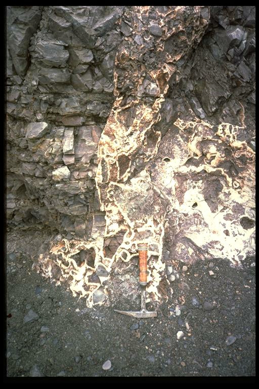
Breccia series: Megabreccia - Breccia - Microbreccia. Because fragments are angular and are displaced, typically very porous and permeable.
Cataclasite is sometimes used to describe fine grained material without fabric and with rather even-size fragments.
Note - formation of breccia involves a dilation, so favoured by low overall pressure, high fluid pressure
Breccia zones are typically permeability conduits in mineralized areas - site of significant economic mineral deposition in hydrothermal systems
But may be cemented with minerals - silica etc, to produce harder, impermeable rock.
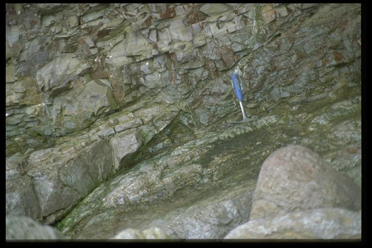
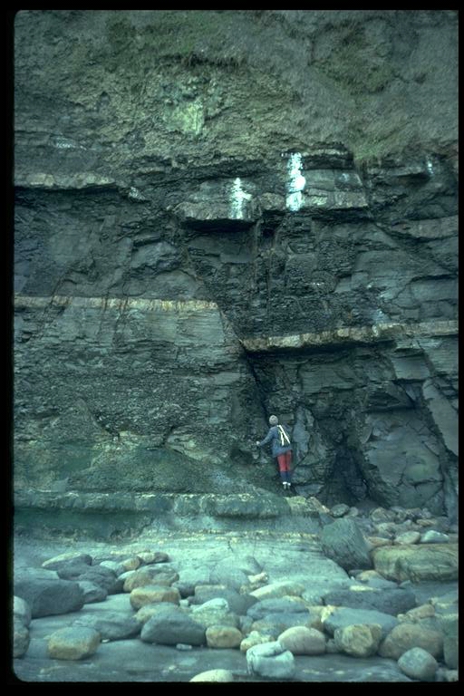
When fault cuts more ductile rocks, typically shales, gouge may form - very fine, grained, and may have some fabric, though typically very variable in orientation.
Photos of gouge 1.2 3 from http://www.geology.washington.edu/~cowan/faultrocks.html
Gouge, unlike breccia and cataclasite, is relatively impermeable.
Modelling gouge production in clay rich successions:
Illustration of oilfield geometry where reservoir contents are dependent on permeability at a fault.
Badley's site is a good source of information on oilfield behaviour of gouge.
Gouge thickness as a function of slip - can gouge be used as an indicator? In a general way only.
Figure from Allmendinger: graph.
Some brittle faults, typically those with very discrete sharp fault planes (no breccia) may be sealed by very fine-grained igneous-looking material. Interpreted as product of melting by frictional heating. This is named pseudotachylite or pseudotachylyte - named after 'tachylite' a very fluid lava
Field photos of pseudotachylite from South Africa, from http://www.lpl.arizona.edu/~rlorenz/pseud.html
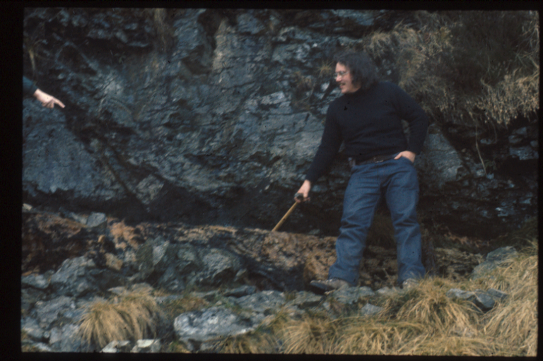
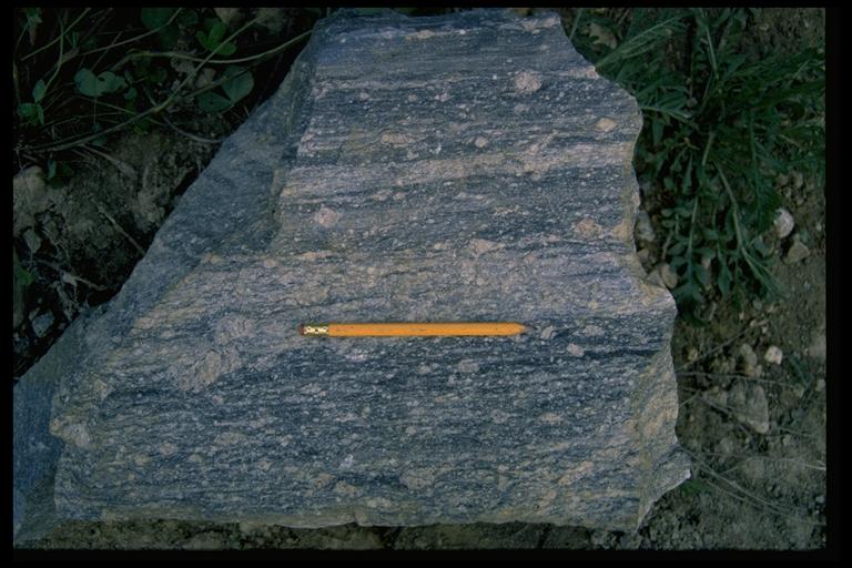
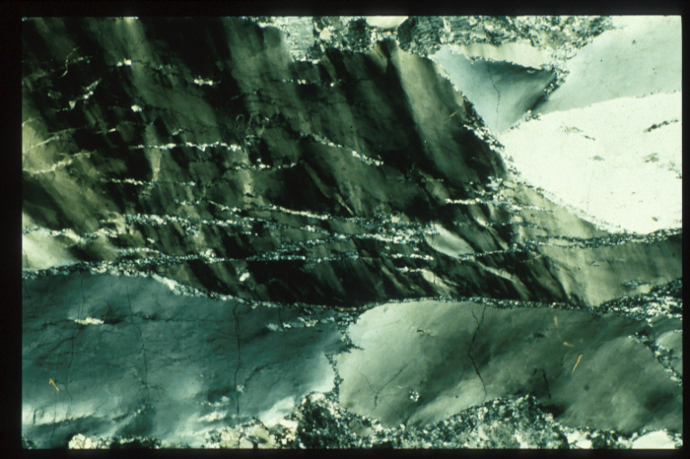
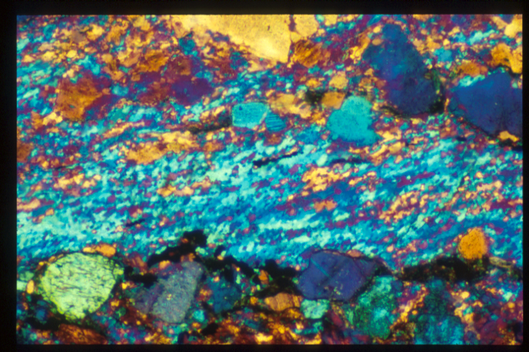
fine grained rocks with fabric from major fault zones...
Caution - name comes from greek word for milling. First interpretation and naming of mylonite was from Moine thrust zone
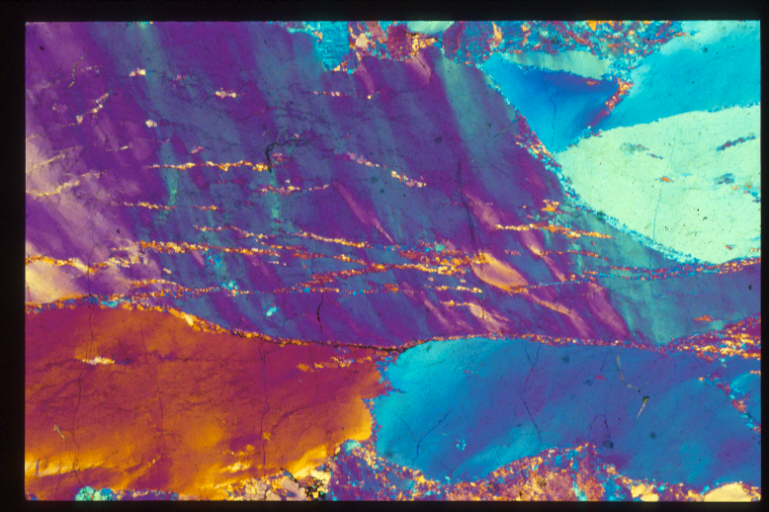
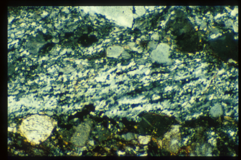
We now know that mylonite is a product of ductile deformation, involving plastic deformation of crystals. Passes through a succession of stages
Photomicrographs of mylonite
Piercing points - these are points where a linear feature intersects the hangingwall and footwall of the fault. They can be simply connected by a slip vector.
Separation plus slip line - In a situation where a slickenline give slip direction, the length of the slip vector may be found by joining points where the same slip line intersects a given surface in the hangingwall and footwall
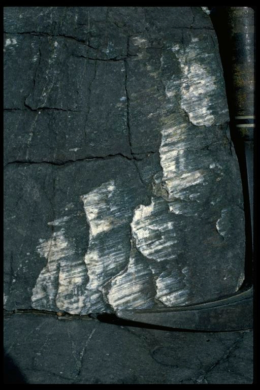
fibres
striations
Fig 4.16 T&M
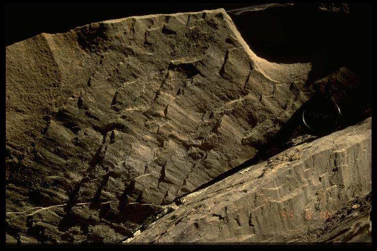
Riedel shears can be related to a stress system where the maximum shear stress is on the fault plane. This plane is at 45° to the principal stresses. Secondary fractures tend to form on either side of the principal compressive stress (typically about 30° from it) Hence the Riedel shears will be located about 15° and 75° from the main fault plane. The 15° shears have the same sense of slip as the main fault and are oriented in the same quadrant as the shortening (P) axis. (ie diverging from the fault in the direction of that the opposing block has moved.) The 75° antithetic Riedel shears have the opposite sense.
See diagram in Twiss and Moores
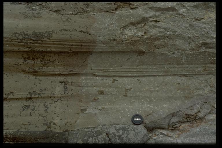
Fabrics
Drag folds
Tight assymetric folds
Porphyroclast systems
Offset folds
Intersecting surfaces
What doesn't work
For a body of rock containing faults, the faults together produce a distortion of the block. Provided the slip is small compared with the spacing between faults, there is a relationship between the strain axes and the slip direction on the fault. The strain axes lie in the movement plane, at 45° to the fault plane (and to the pole to the fault plane). In any given wall, the extension axis points is closer to the movement direction of that wall. The shortening axis lies closer to the movement direction of the opposite wall.
Extension axis is sometimes labelled T, shortening P. Note that these initials are derived from dynamic terms 'Pressure' and 'Tension' - in practice there may be a close relationship between infinitesimal strain and stress orientations, but in principle this terminology blurs the distinction between kinematics and dynamics. Be cautious and don't jump to dynamic conclusions from kinematic data!!!
For arrays of faults, for which movement directions can be determined, it is possible to plot projections showing the extension and shortening axes, contoured.
If the amount of motion on each fault is known, the plots can be weighted according to slip.
Sometimes in a homogeneous body of rock the gouge thickness is used as a proxy for slip.
Also fault strike length can be used as a ballpark proxy for slip, in these calculations
Stress related to faulting can be approached many ways and there are a number of methods available. The simplest make more assumptions , but require fewer data and make fewer assumptions.
P and T axes. We could assume that the extension and shortening axes associated with a given fault are parallel to the stress axes. Hence the extension and shortening kinematic axes are often labelled P and T and treated as the max and min principal stresses (measured with compression positive).
In situations where stress creates faults, different assumptions are appropriate because faults do not in fact form at 45° to stress axes. Experiment tells us that they form at an 'angle of internal friction' theta. Typically about at 30° to the principal compressive stress. So for a stress analysis one method is to place sigma 1 30° from the fault plane not 45.
However, the assumption behind that method may not often be valid. Most bodies of rock have many fractures within them, so arguably most movement in a situation where rocks are stressed may take place on existing fractures. In that case, a given orientation of stress can cause movement on almost any plane, but the direction is determined by the resolved shear stress on a given plane. So one fault plane (with slip sense) could be activated bu a sigma 1 in half of all possible orientations, located in two right dihedra.
Method of right dihedra determines, for every fault in a data set, where are the dihedra that could contain sigma 1. Then for each point in the stereonet we determine how many of these dihedra it lies in. That contour map shows up (ideally) a bullseye around the orientation of sigma 1 that fits the maximum number of fault planes.
Inversion methods: Take a trial orientation and relative magnitude for stress axes, and calculate the resolved shear stress on each fault. Determine an error - difference between the observed slip direction and the direction of shear stress on that surface. Sum the errors in some way. Next, we vary the orientation and relative magnitudes of the stress axes, so as to minimize the error between observation and prediction