
When we move into 3 dimensions we can use analogous measures of strain to those in two dimensions.
The 3 D equivalent of the strain ellipse is the strain ellipsoid. This is the product of deformation applied to a unit sphere.
The orientation of the strain ellipsoid is indicated by the directions of three mutually perpendicular strain axes, which are, in general, the only three lines that are mutually perpendicular before and after deformation.
The strains along the strain axes are the three principal strains. The principal stretches are S1 > S2 > S3 or X, Y, and Z
Cross-sections of the strain ellipsoid are strain ellipses (but there can be circular cross-sections)
Lines of no finite extension typically lie in a cone
Diagram of prolate ellipsoid with lines of no extension
The three strain axes are poles to three principal planes of strain, which are, in general, the only three planes that suffer zero shear strain.
The volume dilation is given by 1+Δ = S1S2S3
To specify the strain ellipsoid completely requires nine numbers:
However, for a non-rotational strain, or if the rotational component of deformation is unknown, only 6 numbers are required because the orientations are the same before and after deformation.
In general, the way we determine the 3D strain ellipsoid is to saw up rocks to define surfaces on which we find 2D strain ellipses. Then recombine the ellipses into an ellipsoid.
The three dimensional deformation gradient tensor is a 3 x 3 matrix.
For a non-rotational strain, the matrix is symmetrical, so only 6 of the numbers are independent.
In 2 dimensions we could specify the shape (distortion component) of the strain ellipse with a single number, the strain ratio.
In 3 dimensions that's not enough. Typically we use two strain ratios to indicate the shape of the ellipsoid. They are conventionally
a = S1/S2 = X/Y
b = S2/S3 = Y/Z
Notice that the minimum value of a and b is 1.0, from the definition.
We can make a plot of a against b, on which the shape of any strain ellipsoid is represented as a point. This is known as a Flynn plot.
Flynn plot VDPM 0416a
Logarithmic Flinn plot or Ramsay diagram VDPM 04
The ratio a/b, known as k, is an indication of the overall symmetry of the strain ellipsoid. Values of k greater than 1 characterize ellipsoids with one long axis and two shorter ones S1 >> S2 > S3, informally known as cigars. Values of k less than 1 characterize ellipsoids with two long axes and one shorter one S1 > S2 >> S3, informally known as pancakes.
If S1 >> S2 = S3 then the strain is described as axially symmetric constriction. k is infinite.
If S1 = S2 >> S3 then the strain is described as axially symmetric flattening. k is zero.
Diagrams of different types of 3D finite strain VDPM 0414
Between the field of cigars (constriction) and the field of pancakes (flattening) is a line where k=1.
If k=1 and we additionally know there is no volume change, then we can make some deductions about strain.
a=b, so S1/S2 = S2/S3
But S1S2S3 = 1 so S2 = 1/S1S3
Substituting for S1 we get S1 = 1/S3 and S2 = 1
Under these circumstances dimensions parallel to S2 remain the same and the only movement of particles due to distortion is in the S1 S3 plane. We can represent this strain as if it were a 2D strain. This type of strain is called plane strain and is a common assumption in section balancing.
Examples of suites of structures under different types of 3D strain.
Rotational deformation is much more complex in 3D than in 2D.
In 2D, the only type of rotation we consider is about an axis perpendicular to the plane of section, and therefore perpendicular to two strain axes.
In 3D, the rotational component of deformation can be perpendicular to two of the strain axes and therefore parallel to the third. When this is the case, the strain is described as monoclinic. The 'before' and 'after' shapes of the strain ellipsoid have the same symmetry as a monoclinic crystal.
However, the rotation axis can be different from any of the strain axes. If this is the case, the strain symmetry of the strain is very low - there is no mirror plane - and the strain is described as triclinic. Triclinic strains, and especially progressive triclinic strains (where rotation and distortion occur concurrently but on different axes) are extremely complicated to work with and require techniqes beyond the scope of this course.
Finite strain is generally the end result of a strain history in which innumberable incremental strains are combined. Defining the complete strain history is a much larger challenge than measuring the finite strain. Nonetheless, in order to understand the way fabrics develop in metamorphic rocks, for example, it is necessary to have an appreciation of strain history. If rocks, and strain, were perfectly homogeneous, we would never be able to figure out strain histories because we would only see the end result of strain. Fortunately, strain partitioning is common. Some components of a rock may respond to the entire strain history whereas others show only part of that history. Careful attention to fabric is often necessary for figuring out strain histories.
In a progressive strain, each increment of strain may, in principle, have a different strain orientation and this makes for an infinite array of strain histories that could produce a given end result. In practice, some types of strain history are more common. For example, if the strain axes coincide with the same material line throughout deformation, then we describe the strain as coaxial. If on the other hand, different material lines behaved as strain axes during different increments, then the strain is non-coaxial.
Diagram of superimposed strain increments VDPM 0409
There are other ways to display different types of strain history. One useful method is using flow lines.
Diagram of flow lines for 4 strain histories
In the coaxial case, flow along the strain axes is directly inward or outward, in a straight line. The strain axes act as flow asymptotes or flow apophyses. They also coincide with the eigenvectors of the strain matrix.
In non-coaxial flow, there can also be flow asymptotes, but they do not usually coincide with the strain axes. (However, flow asymptotes do coincide with the eigenvectors of the deformation matrix). As deformation becomes more non-coaxial the flow asymptotes get closer together, until in the case of simple shear, there is only one asymptote.
The logarithmic Flynn plot, otherwise known as the Ramsay plot, comes into its own in dealing with strain histories. It turns out that is a constant incremental strain is applied, the finite strain follows a straight line path on the Ramsay plot.
In dealing with non-coaxial strains, it would be helpful to have a measure of the amount of rotation compared with distortion. To do this we define a quantity called vorticity.
Consider a rectangular block that undergoes an "infinitesimal" simple shear through a small angleδψ
The infinitesimal strain ellipse is oriented so that S1 and S3 are at 45° to the shear zone boundary.

Like any deformation we can break it down into a pure strain (distortion only) and a rotation.
In this case the deformation is broken down into equal amounts of distortion and rotation.
What do we mean by that?
We can explain simple shear by superimposed infinitesimal increments of distortion (pure strain) and rotation.
The ratio between the rotation and the pure strain is called the vorticity of the deformation.
Vorticity has an effect on the behaviour of the strain axes
In two dimensions, the vorticity is also the cosine of the angle between the flow asymptotes
Diagram of flow lines for 4 strain histories VDPM 0408
Typically, flow converges on one of the strain asymptotes. As strains become large (e.g. in a mylonite) the X axis approaches this asymptote, and all the planar and linear fabric elements tend to converge on this line.
Progressive pure shear is perhaps the simplest case. The diagram shows the effect of progressive pure shear on a rock with competent layers oriented initially perpendicular to S1
As strain starts, competent layers buckle to produce folds. Then, with increasing strain, limbs of the folds rotate from the field of incremental shortening into the field of incremental extension. Initial folds may become unfolded and undergo boudinage.
Geometries like these are extremely common in folded rocks - limbs that are boudinaged while the hinges are tightly buckled.
The situation becomes more complex if layers are initially inclined to the strain axes. If strains become large, folds may rotate towards the stretching direction.
Here's a corresponding diagram for a 'prolate' style of strain. Initially an 'egg-carton' pattern of interfering folds may form. Some of these folds 'unfold' and boudinage may take over.
For this type of symmetric flattening we again show a bed at an initial high angle to the X axis. As strain proceeds, it flattens into the XY plane. Initial folds are unfolded and 'chocolate tablet' boudinage takes over.
Because of their fault-like overall kinematics, the most obvious strain model for a shear zone is simple shear parallel to the boundary.
Diagram of infinitesimal and finite simple shear
This allows the boundary of the shear zone to maintain its length, and therefore to maintain compatibility with adjacent less-strained rock units.
The simple shear may be heterogeneous, provided the shear plane is parallel throughout.
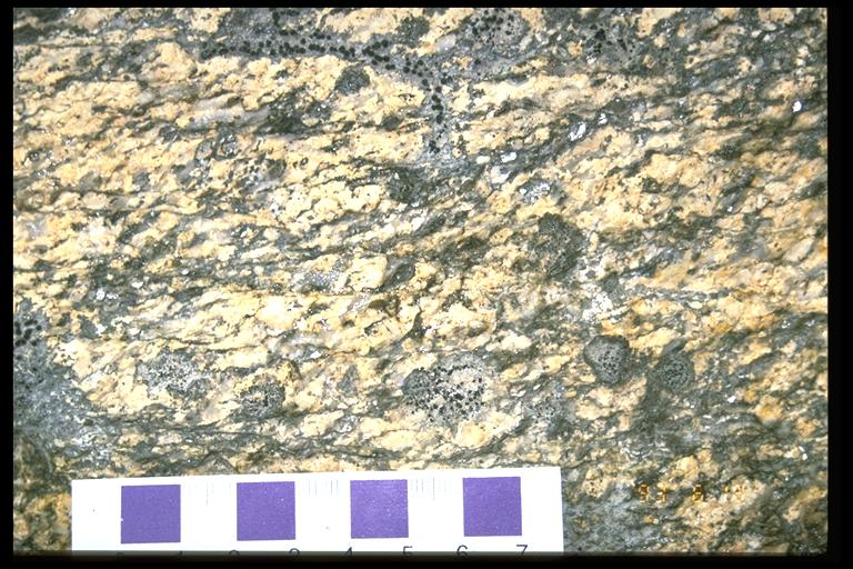
Heterogeneous simple shear VDPM 1215
Photo of heterogeneous shear zone
However, more complex kinematic schemes are possible, but they typically involve either departures from plane strain or volume change. We will consider mostly the simple shear case, but bear in mind that it's an idealized version.
To understand what goes on, we need to look a little more closely at simple shear, and at the distinction between finite and infinitesimal strain.
We are now in a position to think about what happens when we add up all the tiny increments of distortion and rotation that make up a progressive simple shear
 .
.

 snowball (helicitic) garnet
