IV: Kinematics: Strain
Strain basics
Deformation and strain
Kinematic analysis includes
- translation (change in position)
- rotation (change in orientation)
- dilation (change in size) and
- distortion (change in shape)
Strain includes the dilation and distortion components of deformation. In practice, dilation is very difficult to measure in most rocks, and so normally when we speak of strain we are speaking of distortion.
A good way to conceptualize the difference between strain and deformation is to think about a hand sample of deformed rock.
- If the sample was not given an orientation mark when it was collected, the structures in it can only tell you about dilation and distortion (i.e. strain).
- An orientation mark, or observations made in the field, might be able to tell you about rotations and translations too.
Many of the features we see in deformed rocks are products of strain. It is important to have some understanding of strain to answer questions like:
- How is fabric produced by deformation?
- How can we figure out original thicknesses of strata affected by folds and cleavage.
- When we see a major mylonite zone, how much movement has there been
- How much shortening has there been in the Cordillera?
- Can we trust sedimentary structures and paleocurrent directions measured in cleaved rocks?
All these are questions that can only be answered with an understanding of strain.
Pictures of strained rock
What all these have in common is that they have some strain markers: features that had an original shape or size that we can guess, so we can use them to estimate distortion.
Homogeneous and heterogeneous strain
Homogeneous strain is strain that produces the same distortion everywhere. As a result, straight lines stay straight, and parallel lines stay parallel.
Approximately homogeneous strain
Heterogeneous strain is involves distortion or dilation that varies from place to place. Straight lines do not in general stay straight; parallel lines do not in general stay parallel.
Highly heterogeneous strain
When strain is systematically heterogeneous between different components of a rock (e.g. garnets are rotated but quartz is flattened) we describe the strain as partitioned.
Homogeneous strain is much easier to deal with and we will start our study of strain with homogeneous strain. Where we encounter heterogeneous strain, we will still be able to use the concepts and terminology of homogeneous strain by either
- looking at a single point or very small element, or
- by averaging out all the variations and looking at the bulk strain
Strain compatibility
Another phenomenon that helps us understand deformation is strain compatibillity. When rocks deform by ductile processes, it is unusual for large empty spaces to open up within rocks, because of overburden pressure. Hence, the strained portions of a rock have to fit together without leaving any spaces. This limits the types of strain heterogeneity that can occur.
Clearly, not all deformed rocks satisfy strain compatibility. A fault breccia, for example, may contain large open spaces. On the other hand, at large scale, strain compatibility is an important concept in the balancing of cross-sections through thrust belts, so it has applications in both brittle and ductile deformed rocks.
Diagram of balanced cross-section, illustrating strain compatibility
Finite strain, incremental strain, infinitesimal strain, and flow
Everything we have said so far compares an initial state to a final state. Typically, if we look at deformed objects as guides to strain, that's what we are doing.
Diagram of strain paths VDPM 04.05
But in getting from starting state A to final state B, a rock passes through an infinite series of very small steps. There are infinitely many routes that could be followed, of which the diagram shows just two.
Like most physical processes it is sometimes helpful to look at a very small part of the strain history, which is referred to as the incremental strain.
In strain theory, we sometimes consider an infinitesimally small increment of strain, which is referred to as infinitesimal strain. effectively the derivative of the finite strain.
For example, if finite strain is represented by an extension e or a shear strain γ then an incremental strain might be represented δe or δγ infinitesimal strain is de or dγ
de/dt and dγ/dt are strain rates - measures of the speed at which rocks can flow. Typical geological strain rates are of the order of 10-14 per second. Alternatively, the finite strain is the integral of the the infinitesimal strain. We will deal with finite strain first, in 1, 2 and 3 dimensions, reserving our treatment of incremental strain and strain paths for a later section.
Strain in 1 dimension
- In dealing with strain in one dimensin we usually look at material lines. A material line can be thought of as a row of sand grains, or maybe a row of calcium atoms in a calcite crystal. It is a line of material particles (as opposed to a line that is just part of a geometrical construction.)
- Longitudinal strain means change in length. Suppose a material line starts off with length l0 and ends up with length l, we can measure its longitudinal strain in several ways. Photo of stretched belemnites, Map of Andes in South America Stretch from belemnites VDPM 0427
- extension (or fractional change in length) e = (l-l0)/l0
- stretch (new length as a proportion of the old) s = l/l0 = 1+e
- quadratic elongation λ = s2
- natural strain ε = ln(s)
 There is a second way that strain affects material lines. A line is subject to shear strain if adjacent particles of rock flowed past it in a parallel direction. For example, shear strain is occurring at present along the western margin of the North American plate: GPS measurements in western USA
- The easiest way to represent the shear strain along a line is to look for an originally perpendicular material marker line (e.g. in a deformed fossil)
- After deformation we look at how much that marker has rotated out of perpendicular. Again there are several ways to represent the shear strain:
- The angle is the angle of shear represented by the Greek letter psi ψ
- Shear strain (sometimes called engineering shear strain, is represented by the Greek letter gamma γ = tan ψ
- For some purposes it is easier to use the tensor shear strain represented by γ/2
Finite strain in 2 dimensions
Strain ellipse
Once we move into two dimensions, things are a bit more complicated. There are an infinite number of differently oriented material lines in a surface. Lines with different orientations will show different values of S and γ.
The most intuitive way to represent strain in 2D is to imagine a circle before deformation, and to look at its shape after deformation. In general (for homogeneous strain) the circle will become an ellipse - the strain ellipse.
The strain ellipse is the product of a finite strain applied to a circle of unit radius. It is an ellipse whose radius is proportional to the stretch S in any direction.
A deformed circular object has the same shape (though not, strictly, the same size) as the strain ellipse.
Deformed reduction spots
Deformed concretions
If we superimpose the strain ellipse on the original unit circle, we can separate zones of extension from zones of shortening. These zones are separated by lines of no finite extension or LNFE
Diagram of LNFE (=VDPM 04.09)
Depending on the dilation and the shape of the strain ellipse the LNFE may be closer to the long axis or the short axis. If the strain involves a lot of dilation (negative or positive) then all lines may have positive or negative S, and there is no LNFE.
Like any other ellipse, there are two other special lines, the longest and shortest radii, known as strain axes, labelled X and Z or alternatively S1 and S3. (Notice that we are saving S2 and Y for the 3D case.)
The strain axes have another special property - the are perpendicular before and after deformation. So, they must be lines of zero shear strain. In general, they are the only two lines along which the shear strain is zero.
Strain axes perpendicular before and after deformation(= VDPM 0404)
Note that it takes 3 numbers to describe a finite strain in 2D: S1, S3, and the orientation of a strain axis (typically represented φ)
The ratio Rs = S1/ S3 is called the strain ratio and is a measure of the overal intensity of distortion.
The product S1 x S3 is a measure of the dilation.
1 + Δ = S1 x S3
Notice that if we want to extend our description to include the rotational part of deformation (relative to some material reference line like the trace of a horizontal bedding plane or the edge of a shear zone) then we need another measurement - this might be the orientation of the strain axis before deformation (φ0 ).
The difference ω = φ- φ0 is a measure of how much overall rotation has occurred during deformation.
Rotational and non-rotational deformation
Non-rotational deformation or pure strain
Under some circumstances, we may envisage that the strain axes have the same orientation (relative to a reference direction) before and after deformation. Such a deformation is known as a pure strain because the rotation is zero. It is also sometimes called a non-rotational or irrotational deformation. There is a special type of pure strain, known (confusingly) as pure shear in which the dilation is also zero. Then we can say that
1 + Δ = S1 x S3 = 1
and therefore S3 = 1/S1
VDPM 0406 Simple Shear and Pure shear
Rotational deformation
All other types of deformation are termed rotational. In such deformations the strain axes are found to have rotated during deformation.
In general, it is always possible to think of a finite rotational strain as a combination of a non-rotational, pure strain, combined with a simple rotation. (Remember though, that because we are dealing with finite strain, it's not possible using the techniques of this section to say whether the rotation occurred before, during, or after the strain. Often, we assume that rotation and distortion were occurring at the same time, but this is not necessarily the case.) Also note that if we choose our reference direction to coincide with a strain axis, then any finite strain appears non-rotational.
One special case of rotational deformation, simple shear, is of common interest in the study of shear zones and folds. This is a non-dilational strain in which one LNFE is not rotated. Simple shear can easily be simulated by drawing on the side of a deck of cards and then shearing the deck of cards. It is also easily simulated using the shear transformation in CorelDraw or other drawing program.
(VDPM 0406) Simple Shear and Pure shear
Variation of strain with direction:
Mohr circle for strain
In strain analysis we often are able to measure S or γ in a few directions, and would like to reconstruct the strain ellipse from these data.
Example: belemnites
Example: fold and boudinage of veins
Example: veins and stylolites
Example: deformed trilobites
Example: deformed graptolites
To do this, we need to know how S and γ vary with direction in the deformed rock. We measure the direction θ clockwise from the S1 (X) axis, in the deformed rock.
For simplicity, let's deal with a pure strain, so that we don't have to worry about rotation.
The graph of S or e plotted against θ looks like a distorted cosine curve.

(Note that Ramsay's graph uses φ')
We can also plot a graph of shear strain against θ
Plot of shear strain against direction from VDPM fig 04.25
This also looks a bit like a sine wave at low strains, but becomes more distorted at higher strain ratio Rs.
Breddin graphs from text by Ramsay 
In general the mathematical form of these curves makes them rather cumbersome to deal with.
It turns out that there's a simplification that can be achieved if we define two new quantities, based on the square of the stretch, also known as the quadratic elongation λ.
The values of λ along the strain axes are λ1 and λ3.
λ' is defined as 1/λ and γ' is defined as γ/λ
Then

and

These are equations of a circle with radius (λ'3 - λ'1)/2 with centre at (λ'3 + λ'1)/2
[Note - VDPM use phi where JW diagram uses theta.]
Notice how any point on the Mohr circle describes the state of strain on a line in the strained rock. It is easy to convert from λ' and γ' to the more useful quantities S and γ, and vice versa. Notice also that angles θ measured in the rock are represented by points on the circle that are at an angle 2θ around the Mohr circle. The two strain axes, 90° apart in the rock, are located 180° apart on the circle. Notice that γ', and therefore γ, is zero (as it should be) at both these axes.
In addition, the angle marked ψ on the diagram has to be tan-1 (γ'/λ') = tan-1 γ, or the angle of shear.
Because it can be easily constructed with a compass, the Mohr circle construction is very useful for determining longitudinal strain and shear strain in any given direction, provided the principal strains are known.
Deformation matrix
Definition
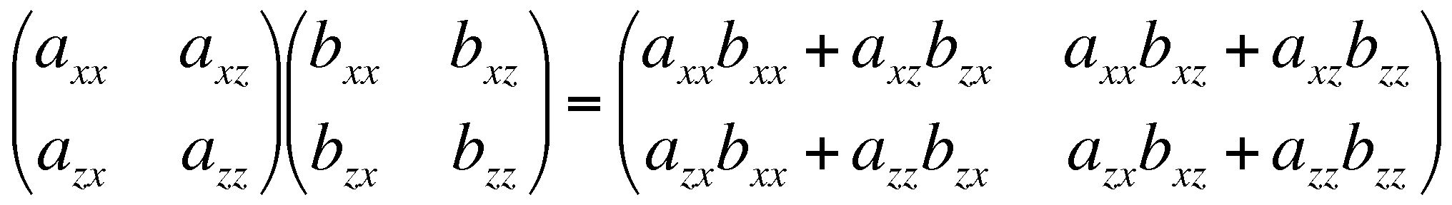
So far we have met two methods for representation of finite strain in 2D. These are the Mohr circle and the strain ellipse. We now introduce a third representation, that is actually the basis for all the theory of the strain ellipse and the Mohr circle. This is a 2 x 2 matrix of 4 numbers known as the deformation gradient tensor, or more simply as the deformation matrix and commonly represented with a bold F.
- We can draw a unit square, and set up some axes so that it is at the origin of a graph. The square will have two diagonally opposite corners at coordinates (1,0) and (0,1).
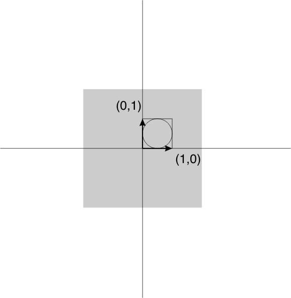
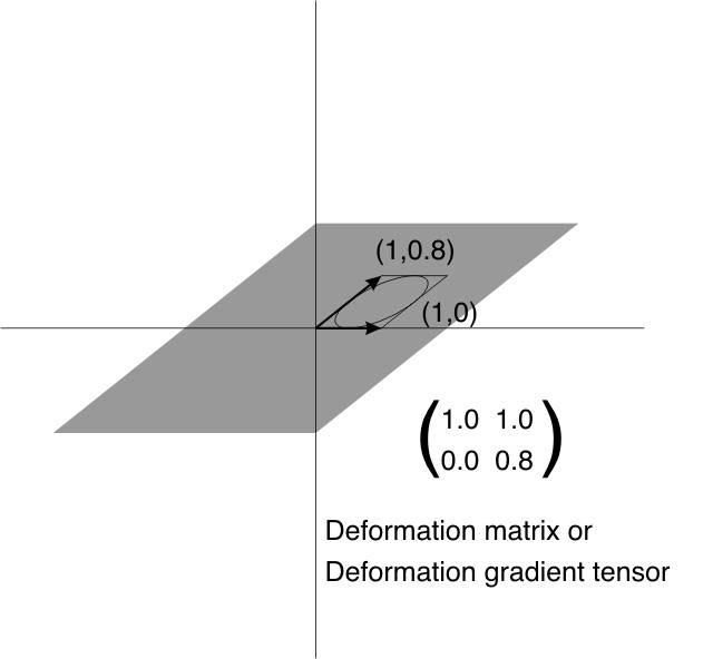
- After deformation the square will be a parallelogram. The coordinates of the two diagonally opposite corners are used to fill the deformation matrix, also known as the deformation gradient tensor.
Using the deformation matrix to simulate strain
A vector is just a one-column matrix. If a vector is used to represent the coordinates of a point in space, then matrix multiplication may be used to transform that point to a new location.
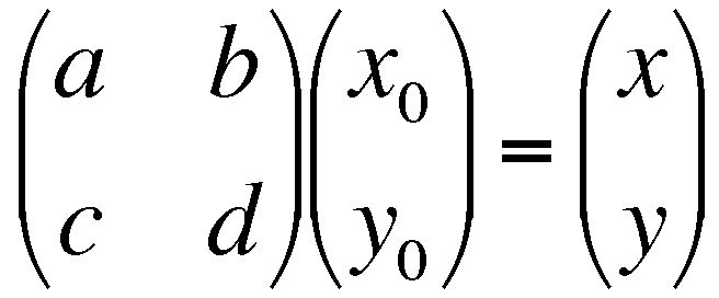
This can also be written Fx0 = x
Finite strain in 3D
Strain ellipsoid and tensor
When we move into 3 dimensions we can use analogous measures of strain to those in two dimensions.
The 3 D equivalent of the strain ellipse is the strain ellipsoid. This is the product of deformation applied to a unit sphere.
The orientation of the strain ellipsoid is indicated by the directions of three mutually perpendicular strain axes, which are, in general, the only three lines that are mutually perpendicular before and after deformation.
The three strain axes are poles to three principal planes of strain, which are, in general, the only three planes that suffer zero shear strain.
The strains along the strain axes are the three principal strains. The principal stretches are S1 > S2 > S3 or X, Y, and Z
The volume dilation is given by 1+Δ = S1S2S3
To specify the strain ellipsoid completely requires nine numbers:
- The three values of S1 S2 S3
- The plunge and trend of one strain axis after deformation
- The rake of a second axis in the plane perpendicular to the first. (The third axis is mutually perpendicular to the other two).
- The plunge trend and rake for the three axes before deformation
However, for a non-rotational strain, or if the rotational component of deformation is unknown, only 6 numbers are required because the orientations are the same before and after deformation.
The three dimensional deformation gradient tensor is a 3 x 3 matrix.
For a non-rotational strain, the matrix is symmetrical, so only 6 of the numbers are independent.
Cross-sections of the strain ellipsoid are strain ellipses (but there can be circular cross-sections)
Lines of no finite extension typically lie in a cone
Diagram of prolate ellipsoid with lines of no extension
Strain ellipsoid shapes
In 2 dimensions we could specify the shape (distortion component) of the strain ellipse with a single number, the strain ratio.
In 3 dimensions that's not enough. Typically we use two strain ratios to indicate the shape of the ellipsoid. They are conventionally
a = S1/S2 = X/Y
b = S2/S3 = Y/Z
Notice that the minimum value of a and b is 1.0, from the definition that specifies . We can make a plot of a against b, on which the shape of any strain ellipsoid is represented as a point. This is known as a Flynn plot.
Flynn plot VDPM 0416a

The ratio a/b, known as k, is an indication of the overall symmetry of the strain ellipsoid. Values of k greater than 1 characterize ellipsoids with one long axis and two shorter ones S1 >> S2 > S3, informally known as cigars. Values of k less than 1 characterize ellipsoids with two long axes and one shorter one S1 > S2 >> S3, informally known as pancakes.
If S1 >> S2 = S3 then the strain is described as axially symmetric constriction.
If S1 = S2 >> S3 then the strain is described as axially symmetric flattening.
Between the field of cigars (constriction) and the field of pancakes (flattening) is a line where k=1.
If k=1 and we additionally know there is no volume change, then we can make some deductions about strain.
a=b, so S1/S2 = S2/S3
But S1S2S3 = 1 so S2 = 1/S1S3
Substituting for S1 we get S1 = 1/S3 and S2 = 1
Under these circumstances dimensions parallel to S2 remain the same and the only movement of particles due to distortion is in the S1 S3 plane. We can represent this strain as if it were a 2D strain. This type of strain is called plane strain and is a common assumption in section balancing.
Logarithmic Flinn plot or Ramsay diagram
Examples of suites of structures under different types of 3D strain.
Rotation and strain in 3D
Rotational deformation is much more complex in 3D than in 2D.
In 2D, the only type of rotation we consider is about an axis perpendicular to the plane of section, and therefore perpendicular to two strain axes.
In 3D, the rotational component of deformation can be perpendicular to two of the strain axes and therefore parallel to the third. When this is the case, the strain is described as monoclinic. The 'before' and 'after' shapes of the strain ellipsoid have the same symmetry as a monoclinic crystal.
However, the rotation axis can be different from any of the strain axes. If this is the case, the strain symmetry of the strain is very low - there is no mirror plane - and the strain is described as triclinic. Triclinic strains, and especially progressive triclinic strains (where rotation and distortion occur concurrently but on different axes) are extremely complicated to work with and require techniqes beyond the scope of this course.
Measuring strain in 2D
We now have enough information to deal with practical measurement of strain from rocks.
Most methods for measuring strain directly in rocks work in 2D. In general, the way we determine the 3D strain ellipsoid is to saw up rocks to define surfaces on which we find 2D strain ellipses. Then recombine the ellipses into an ellipsoid.
It's important to remember that any strain determination is dependent on some assumptions about the starting state of the rock.
Because the starting rock can no longer be examined, these assumptions are difficult to test.
In strain analysis the best strategy is to use 2 or more different techniques, based on different assumptions, and see if they give the same answer.
Direct measurement of elliptical objects
Deformed reduction spots
This is the simplest case. If we have an object that was perfectly circular before deformation, we can measure its shape to obtain the shape of the strain ellipse. The most likely objects are volcanic lapilli, and reduction spots.
The starting assumptions are
- The objects were initially spherical
- They deformed homogeneously with the matrix
Because we typically have no control over original size, this method can only tell us about distortion, not dilation.
Limestone ooids are sometimes very close to circular. However, they are less likely to deform homogenenously with their matrix, because they often have slightly different texture or composition than the surrounding material.
Direct measurement of longitudinal strain
Belemnites
Burrows
Tourmaline crystals
Linear objects are sometimes available, in circumstances where we can reconstruct the length before deformation. For example, very rigid elongated objects such as belemnite fossils and toumaline crustals [pictures from Ramsay and Huber] my undergo boudinage during strain. It is possible to determine the original length of the object by adding up the lengths of all the boudins. The final length can be measured directly, and the stretch can be calculated (l/l0).
Stretch from belemnites VDPM 0427
Once several objects have been measured, their orientations and lengths can be plotted (in radial coordinates). A best fit ellipse may be estimated using a set of elliptical templates. In theory a minimum of three points may constrain the ellipse but usually more are advisable.
The assumptions for this method are:
- There is no distortion of the boudins
- The separation of the boudins represents the whole of the longitudinal strain.
If these assumptions are satisfied, this method can in theory yield both the dilational and distortional components of the strain ellipse.
Measurement of shear strain: Mohr circle and Wellman methods
Fossils
Trilobite
Often, we can measure shear strains more easily than longitudinal strains. This is particularly the case with bilaterally symmetrical fossils, which have been distorted by strain. A minimum of two, differently oriented fossils is necessary. If only two or three fossils are available, a Mohr circle construction is typically used. For multiple measurements we use a construction called a Wellman plot.
For the Mohr construction, plot the circular part of a Mohr diagram at arbitrary size on tracing paper. Draw two radii representing the lines along which shear strain is known; the angle between the radii must be double the angle in the rock (because angles are doubled in the Mohr construction). Next, plot the axes on graph paper, and draw lines from the origin inclined at angles ψ to the horizontal axis. Then superimpose the tracing paper on the graph paper to complete the construction, making sure that corresponding lines intersect.
For the Wellman plot, first draw on tracing paper a horizontal reference line. For each fossil, measure the orientations of two originally perpendicular lines. Draw lines with the same orientation, starting at each end of the reference line (4 lines in all, forming a parallelogram). Mark the corners of the parallelogram. Repeat for each fossil. The marked points should fall on a strain ellipse that has the reference line as a radius.
Wellman technique
Assumptions for this method:
- Original shape of fossils is known
- Fossils have deformed homogeneously with their matrix
This method yields only the shape (distortion component) and not the size (dilation component) of the strain ellipse.
Fry's method
There are many examples of rocks in which the only strain markers are objects which are expected not to have deformed homogeneously with their matrix. Examples include pebbles in conglomerates with a soft matrix, sand grains or ooids that have become sutured by stylolytic contacts, etc.
[ooids bounded by stylolites].
In these cases, the shapes of the objects cannot be used to determine strain. Instead, it may be possible to use the spacing of the objects. This method works if the objects were uniformly spaced in all directions before deformation, or if they were at least, statistically uniform in their spacing. (What this means is that it's possible to identify an average or typical spacing of nearest objects, measured centre to centre, in the undeformed rock.)
The procedure again involves tracing paper. Mark an x or a set of axes on tracing paper. Place the origin over one object. Mark the centres of all nearby objects. Move the tracing paper to the next object (without rotating it). Repeat the procedure.
Fry method VDPM 0423
After a sufficient number of objects has been traced (typically >50), an elliptical anticluster may appear in the centre of the diagram. The shape of this anticluster is the shape of the strain ellipse.
Assumptions for this method
- Objects were initially uniformly and isotropically distributed
- If objects were not spherical, they did not have a preferred original orientation
- Objects have not slid past each other during deformation
Unless the original size of objects can be estimated (rarely possible) this method gives only the shape (distortion component) of the strain ellipse.
Rf/φ methods
A common problem in strain analysis may be that the only available markers were elliptical, not circular, even before deformation. We can attempt to overcome this with a plot known as an Rf/φ plot.
Rf is the ellipticity of a measured object (e.g. the ratio of long axis to short axis of a deformed pebble.). Rf can be thought of as a combination of an initial ellipticity Ri and a strain ellipticity Rs.
Phi is the orientation of the long axis of the object, with respect to some reference direction (e.g. north, or in a vertical section, horizontal.)
Deformed pebbles 1
Pebbles 2
RfPhi Plot JW diagram
RfPhi VDPM
In the plot, each point is plotted on axes Rf and φ, typically producing a scattered cluster. The centre of the cluster represents the φ value of the S1 axis. The value of Rs is represented by Rf at the densest part of the cluster. Sets of standardized curves are available for estimating Rs.
Map of Morcles Nappe
View of Morcles Nappe
Another view
Strain distribution in Morcles Nappe VDPM 0415b
[Another version]
[Alternatively, the two can be plotted on a hyperbolic net, in which φ is measured as an angle and Rf is plotted as a distance from the centre. The net is rotated so that its line of symmetry bisects the cluster. The net also shows a set of hyperbolic lines; the line which bisects the cluster is chosen, and the value of R at its closest approach to the origin is an estimate of Rs.]
Waldron's method
[Powerpoint presentation on Meguma Terrane]
Restoring oriented structures in deformed rocks
A typical example of a retrodeformation problem is a slate belt in which the orientations of sedimentary structures have been measured. Some analyses of sedimentary structures are carried out by simple rotation of the structures to horizontal. This works well if bedding surfaces are surfaces of no strain (in flexural slip folding) for example.
More usually there is significant strain in bedding surfaces of deformed rocks, and to get a picture of paleocurrent distributions it is necessary to remove the effects of strain.
Effectively, this means applying a strain which is the opposite of the finite strain, to each measurement. The method used depends on the way in which strain has been determined.
If the strain ellipse has been determined
Diagram
We know
- Strain ratio Rs,
- Orientation of the strain axis φ.
Measure the angle between the structure and the long axis of the strain ellipse in the deformed state θ'.
To restore this angle to the original state, calculate θ according to the formula
Strain ratio Rs = tanθ/tanθ'
After removing the distortion by this formula, restore the rotational component of deformation (if known) by simple rotation.
If the deformation matrix has been determined
F=
Calculate the reciprocal deformation matrix:
Actually, because only the distortion matters for rotation, it's possible to ignore the dilation. If we assume the dilation ab-cd = 1 then the simplified reciprocal matrix becomes 
Multiply each vector by this matrix to restore it to an original orientation.
Examples
Here are examples from the Meguma Group of NS showing the reorientation of paleocurrents
Eastern shore
South shore
Measuring strain in 2D
We now have enough information to deal with practical measurement of strain from rocks. It's important to remember that any strain determination is dependent on some assumptions about the starting state of the rock.
Because the starting rock can no longer be examined, these assumptions are difficult to test.
In strain analysis the best strategy is to use 2 or more different techniques, based on different assumptions, and see if they give the same answer.
Direct measurement of elliptical objects
Deformed reduction spots
This is the simplest case. If we have an object that was perfectly circular before deformation, we can measure its shape to obtain the shape of the strain ellipse. The most likely objects are volcanic lapilli, and reduction spots.
The starting assumptions are
- The objects were initially spherical
- They deformed homogeneously with the matrix
Because we typically have no control over original size, this method can only tell us about distortion, not dilation.
Limestone ooids are sometimes very close to circular. However, they are less likely to deform homogenenously with their matrix, because they often have slightly different texture or composition than the surrounding material.
Direct measurement of longitudinal strain
Belemnites
Burrows
Tourmaline crystals
Linear objects are sometimes available, in circumstances where we can reconstruct the length before deformation. For example, very rigid elongated objects such as belemnite fossils and toumaline crustals [pictures from Ramsay and Huber] my undergo boudinage during strain. It is possible to determine the original length of the object by adding up the lengths of all the boudins. The final length can be measured directly, and the stretch can be calculated (l/l0).
Stretch from belemnites VDPM 0427
Once several objects have been measured, their orientations and lengths can be plotted (in radial coordinates). A best fit ellipse may be estimated using a set of elliptical templates. In theory a minimum of three points may constrain the ellipse but usually more are advisable.
The assumptions for this method are:
- There is no distortion of the boudins
- The separation of the boudins represents the whole of the longitudinal strain.
If these assumptions are satisfied, this method can in theory yield both the dilational and distortional components of the strain ellipse.
Measurement of shear strain: Mohr circle and Wellman methods
Fossils
Trilobite
Often, we can measure shear strains more easily than longitudinal strains. This is particularly the case with bilaterally symmetrical fossils, which have been distorted by strain. A minimum of two, differently oriented fossils is necessary. If only two or three fossils are available, a Mohr circle construction is typically used. For multiple measurements we use a construction called a Wellman plot.
For the Mohr construction, plot the circular part of a Mohr diagram at arbitrary size on tracing paper. Draw two radii representing the lines along which shear strain is known; the angle between the radii must be double the angle in the rock (because angles are doubled in the Mohr construction). Next, plot the axes on graph paper, and draw lines from the origin inclined at angles ψ to the horizontal axis. Then superimpose the tracing paper on the graph paper to complete the construction, making sure that corresponding lines intersect.
For the Wellman plot, first draw on tracing paper a horizontal reference line. For each fossil, measure the orientations of two originally perpendicular lines. Draw lines with the same orientation, starting at each end of the reference line (4 lines in all, forming a parallelogram). Mark the corners of the parallelogram. Repeat for each fossil. The marked points should fall on a strain ellipse that has the reference line as a radius.
Wellman technique
Assumptions for this method:
- Original shape of fossils is known
- Fossils have deformed homogeneously with their matrix
This method yields only the shape (distortion component) and not the size (dilation component) of the strain ellipse.
Fry's method
There are many examples of rocks in which the only strain markers are objects which are expected not to have deformed homogeneously with their matrix. Examples include pebbles in conglomerates with a soft matrix, sand grains or ooids that have become sutured by stylolytic contacts, etc.
[ooids bounded by stylolites].
In these cases, the shapes of the objects cannot be used to determine strain. Instead, it may be possible to use the spacing of the objects. This method works if the objects were uniformly spaced in all directions before deformation, or if they were at least, statistically uniform in their spacing. (What this means is that it's possible to identify an average or typical spacing of nearest objects, measured centre to centre, in the undeformed rock.)
The procedure again involves tracing paper. Mark an x or a set of axes on tracing paper. Place the origin over one object. Mark the centres of all nearby objects. Move the tracing paper to the next object (without rotating it). Repeat the procedure.
Fry method VDPM 0423
After a sufficient number of objects has been traced (typically >50), an elliptical anticluster may appear in the centre of the diagram. The shape of this anticluster is the shape of the strain ellipse.
Assumptions for this method
- Objects were initially uniformly and isotropically distributed
- If objects were not spherical, they did not have a preferred original orientation
- Objects have not slid past each other during deformation
Unless the original size of objects can be estimated (rarely possible) this method gives only the shape (distortion component) of the strain ellipse.
Rf/φ methods
A common problem in strain analysis may be that the only available markers were elliptical, not circular, even before deformation. We can attempt to overcome this with a plot known as an Rf/φ plot.
Rf is the ellipticity of a measured object (e.g. the ratio of long axis to short axis of a deformed pebble.). Rf can be thought of as a combination of an initial ellipticity Ri and a strain ellipticity Rs.
Phi is the orientation of the long axis of the object, with respect to some reference direction (e.g. north, or in a vertical section, horizontal.)
Deformed pebbles 1
Pebbles 2
RfPhi Plot JW diagram
RfPhi VDPM
In the plot, each point is plotted on axes Rf and φ, typically producing a scattered cluster. The centre of the cluster represents the φ value of the S1 axis. The value of Rs is represented by Rf at the densest part of the cluster. Sets of standardized curves are available for estimating Rs.
Map of Morcles Nappe
View of Morcles Nappe
Another view
Strain distribution in Morcles Nappe VDPM 0415b
[Another version]
[Alternatively, the two can be plotted on a hyperbolic net, in which φ is measured as an angle and Rf is plotted as a distance from the centre. The net is rotated so that its line of symmetry bisects the cluster. The net also shows a set of hyperbolic lines; the line which bisects the cluster is chosen, and the value of R at its closest approach to the origin is an estimate of Rs.]
Waldron's method
[Powerpoint presentation on Meguma Terrane]
Restoring oriented structures in deformed rocks
A typical example of a retrodeformation problem is a slate belt in which the orientations of sedimentary structures have been measured. Some analyses of sedimentary structures are carried out by simple rotation of the structures to horizontal. This works well if bedding surfaces are surfaces of no strain (in flexural slip folding) for example.
More usually there is significant strain in bedding surfaces of deformed rocks, and to get a picture of paleocurrent distributions it is necessary to remove the effects of strain.
Effectively, this means applying a strain which is the opposite of the finite strain, to each measurement. The method used depends on the way in which strain has been determined.
If the strain ellipse has been determined
Diagram
We know
- Strain ratio Rs,
- Orientation of the strain axis φ.
Measure the angle between the structure and the long axis of the strain ellipse in the deformed state θ'.
To restore this angle to the original state, calculate θ according to the formula
Strain ratio Rs = tanθ/tanθ'
After removing the distortion by this formula, restore the rotational component of deformation (if known) by simple rotation.
If the deformation matrix has been determined
F=
Calculate the reciprocal deformation matrix:
Actually, because only the distortion matters for rotation, it's possible to ignore the dilation. If we assume the dilation ab-cd = 1 then the simplified reciprocal matrix becomes
Multiply each vector by this matrix to restore it to an original orientation.
Examples
Here are examples from the Meguma Group of NS showing the reorientation of paleocurrents
Eastern shore
South shore
Progressive strain and flow
Finite strain is generally the end result of a strain history in which innumberable incremental strains are combined. Defining the complete strain history is a much larger challenge than measuring the finite strain. Nonetheless, in order to understand the way fabrics develop in metamorphic rocks, for example, it is necessary to have an appreciation of strain history. If rocks, and strain, were perfectly homogeneous, we would never be able to figure out strain histories because we would only see the end result of strain. Fortunately, strain partitioning is common. Some components of a rock may respond to the entire strain history whereas others show only part of that history. Careful attention to fabric is often necessary for figuring out strain histories.
Protomylonite with C-S fabric
Coaxial and non-coaxial strain histories
In a progressive strain, each increment of strain may, in principle, have a different strain orientation and this makes for an infinite array of strain histories that could produce a given end result. In practice, some types of strain history are more common. For example, if the strain axes coincide with the same material line throughout deformation, then we describe the strain as coaxial. If on the other hand, different material lines behaved as strain axes during different increments, then the strain is non-coaxial.
Diagram of superimposed strain increments VDPM 0409
There are other ways to display different types of strain history. One useful method is using flow lines.
Diagram of flow lines for 4 strain histories
In the coaxial case, flow along the strain axes is directly inward or outward, in a straight line. The strain axes act as flow asymptotes or flow apophyses. They also coincide with the eigenvectors of the strain matrix.
In non-coaxial flow, there can also be flow asymptotes, but they do not usually coincide with the strain axes. (However, flow asymptotes do coincide with the eigenvectors of the deformation matrix). As deformation becomes more non-coaxial the flow asymptotes get closer together, until in the case of simple shear, there is only one asymptote.
The logarithmic Flynn plot, otherwise known as the Ramsay plot, comes into its own in dealing with strain histories. It turns out that is a constant incremental strain is applied, the finite strain follows a straight line path on the Ramsay plot.
Rotation and vorticity
In dealing with non-coaxial strains, it would be helpful to have a measure of the amount of rotation compared with distortion. To do this we define a quantity called vorticity.
Consider a rectangular block that undergoes an "infinitesimal" simple shear through a small angleδψ
The infinitesimal strain ellipse is oriented so that S1 and S3 are at 45° to the shear zone boundary.

Diagram
Like any deformation we can break it down into a pure strain (distortion only) and a rotation.
In this case the deformation is broken down into equal amounts of distortion and rotation.
What do we mean by that?
- Suppose that the small distortion represented here had S1 = 1.05 and S2=.95, then we could say that is 5% distortion.
- The rotation part of the deformation, for simple shear, would be .05 radian.
We can explain simple shear by superimposed infinitesimal increments of distortion (pure strain) and rotation.
The ratio between the rotation and the pure strain is called the vorticity of the deformation.
- For progressive simple shear vorticity is 1.
- For progressive pure shear vorticity is zero.
- Vorticity can locally be greater than 1, eg in delta structures and snowball garnets.
Vorticity has an effect on the behaviour of the strain axes
- When the vorticity is zero, the strain axes have constant direction relative to lines of rock particles. The strain is coaxial
- When vorticity is non-zero, the lines of rock particles rotate through the strain axes. The strain is non-coaxial.
In two dimensions, the vorticity is also the cosine of the angle between the flow asymptotes
Diagram of flow lines for 4 strain histories VDPM 0408
Typically, flow converges on one of the strain asymptotes. As strains become large (e.g. in a mylonite) the X axis approaches this asymptote, and all the planar and linear fabric elements tend to converge on this line.
Examples of progressive strain paths
Progressive coaxial strains
Progressive pure shear
Progressive pure shear is perhaps the simplest case. The diagram shows the effect of progressive pure shear on a rock with competent layers oriented initially perpendicular to S1
As strain starts, competent layers buckle to produce folds. Then, with increasing strain, limbs of the folds rotate from the field of incremental shortening into the field of incremental extension. Initial folds may become unfolded and undergo boudinage.
Diagram
Geometries like these are extremely common in folded rocks - limbs that are boudinaged while the hinges are tightly buckled.
The situation becomes more complex if layers are initially inclined to the strain axes. If strains become large, folds may rotate towards the stretching direction.
Diagram
Progressive axially symmetric extension
Diagram
Here's a corresponding diagram for a 'prolate' style of strain. Initially an 'egg-carton' pattern of interfering folds may form. Some of these folds 'unfold' and boudinage may take over.
Progressive axially symmetric shortening
Diagram
For this type of symmetric flattening we again show a bed at an initial high angle to the X axis. As strain proceeds, it flattens into the XY plane. Initial folds are unfolded and 'chocolate tablet' boudinage takes over.
Progressive non-coaxial strain
Progressive simple shear
Because of their fault-like overall kinematics, the most obvious strain model for a shear zone is simple shear parallel to the boundary.
Diagram of infinitesimal and finite simple shear
This allows the boundary of the shear zone to maintain its length, and therefore to maintain compatibility with adjacent less-strained rock units.
The simple shear may be heterogeneous, provided the shear plane is parallel throughout.
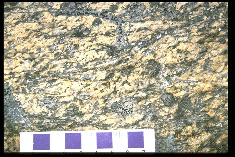
Heterogeneous simple shear VDPM 1215
Photo of heterogeneous shear zone
However, more complex kinematic schemes are possible, but they typically involve either departures from plane strain or volume change. We will consider mostly the simple shear case, but bear in mind that it's an idealized version.
To understand what goes on, we need to look a little more closely at simple shear, and at the distinction between finite and infinitesimal strain.
- We draw a diagram of a sheared card deck to illustrate simple shear - this is a finite simple shear. Described this way, the rock could have taken any strain path to get from its original state to its sheared state.
- However, if it's in a shear zone, probably every part of the strain was a simple shear. The strain going on at any instant was infinitesimal simple shear.
- We describe the overall history as a progressive simple shear.
We are now in a position to think about what happens when we add up all the tiny increments of distortion and rotation that make up a progressive simple shear
 .
.
- The infinitesimal strain axes are always at 45° to the shear zone boundary.
- The lines of no infinitesimal extension are always parallel and perpendicular to the shear zone boundary.
- The finite strain axes rotate with the vorticity, gradually falling down towards the shear plane.
- If the angle of S1 to the shear zone is θ and the amount of simple shear is γ, then γ = 2 / tan(2θ).
- The lines of no finite extension get closer to each other on either side of the S1 axis. One of these lines is always parallel to the shear zone boundary.
Structures typical of shear zones:
- Veins
- Consider what happens to a vein that opens up in a shear zone in response to high fluid pressure.
- Veins are most likely to open in an orientation perpendicular to the infinitesimal S1.
- Initially such a vein is in a field of infinitesimal shortening, so it may tend to fold.
- However it also rotates with the vorticity, and once it passes through perpendicular to the SZB it will start to extend again. A previously folded vein may tend to unfold or it may undergo boudinage as it extends.
- Layers
- Layers and fold limbs may rotate from the field of shortening into the field of extension
- Folds formed early in strain history may change their symmetry during shear
- Folds may become repetedly refolded
- Folds may be rotated towards the extension direction, producing sheath-like geometry.
- Simple Fabrics
- Strain sensitive fabrics rotate with the finite strain. Examples include stretching lineations, and foliations defined by flattened objects.
- Strain insensitive fabrics are fabrics that form in response to small strain increments, and therefore are aligned parallel to the infinitesimal strain not the finite strain. Under the microscope, many rocks in shear zones show microscopic oblique foliation (accessory plate) - crystal long axes at about 45° to the shear zone, that seems to keep this orientation despite variations in finite strain. The minerals must continuously recrystallize so as to stay aligned close to the infinitesimal strain axes.
- View with accessory plate
- Strain partitioning and composite fabrics
- Heterogeneities in the angle of shear lead to the development of small intensely sheared zones, called C-planes if they are parallel to the shear zone boundary, or called extensional crenulation if they are inclined so that they extend the foliations. Intervening zones that have smaller amounts of strain are characterized by foliation that is highly oblique to the SZB, known as S-foliation. The combination of C and S planes is one of the most widespread indications of shear sense.
- It is also common to see partitioning of the rotational and non-rotational parts of the strain, particularly when there are resistant, equant mineral grains which can roll more easily than they are distorted. These grains tend to focus vorticity, producing delta structures and or textures.


